Congestion Control

Congestion occurs if two packets arrive at the the router at the same time. The router will transmit one and buffer or drop the other. This occurs more often when the internet traffic is bursty, causing many packets to arrive close in time, resulting in packet delays and drops.

Root cause: statistical multiplexing. This is the main region for congestion because there's too many nodes in the network.

Two basic questions:

1. how does the sender detect congestion?
2. how does the sender adjust its sending rate? It needs to adjust it to address these three objectives: 1) find available bottleneck bandwidth so it doesn't exceed the it, 2) adjust to bandwidth variation, like how much network is available at that moment 3) and we want to share the bandwidth because there are multiple TCP connections/users, so we don't want to take up everything.

The congestion collapse occurred in October 1986.

• At this time, the sending rate was only limited by flow control. This meant that when there were dropped packets, senders would repeatedly retransmit.
• This led to the "congestion collapse", where the throughput on the NSF network dropped from 32K bits/s to 40 bits/s.
• This was "fixed" by Van Jacobson's development of TCP's congestion control (CC) algorithms.

Jacobson's fix

Jacobson's fix to TCP was to extend the TCP's existing window-based protocol but adapt the window size in response to congestion.

• This was a pragmatic and effective solution because it required no upgrades to routers or applications, backwards compatible, and the patch required only a few lines of code to TCP implementations.

Nowadays with data centers and cloud services, congestion control problems are extensively researched and improved upon.

Key design consideration:

• How do we know there's a congestion?
  • We know that a network is congested when there are implicit and/or explicit signals from the network
• Who takes care of congestion?
  • Congestion is the responsibility of the end hosts (may receive some help from the network).
• How do we handle congestion?
  • Congestion is handled via continuous adaption.

Three issues to consider:

• discovering the available (bottleneck) bandwidth.
• adjust the variation in bandwidth
• sharing bandwidth between flows or different end hosts.

Simple two host example: A is the sending host, B is the receiving host, and there's a buffer in the router that can be modeled as a single queue.

• The first issue is we don't know the available bandwidth. It could be a gigabit link, or it could be a modem. However, with no prior knowledge, we can't pick a sending rate to match the bottleneck bandwidth.
• So, we need to adjust to match the instantaneous bandwidth (assuming you have a rough idea of bandwidth)

There are two issues when considering multiple flows and sharing bandwidth. Imagine a couple senders and a couple receivers:

• adjust total sending rate to match the bandwidth
• allocation of bandwidth between flows

This is a better reflection of reality, where congestion control is a resource allocation problem involving many flows, many links, and complicated global dynamics.

Approaches in designing a congestion control:

1. send without care. we don't know the capacity of the network, and we send what ever we have without care about the congestion. This is what we had before 1980s.
   1. cons: many packet drops
2. Reserve some of the resources/links and try to use this reserve capacity.
   1. cons: you must pre-arrange bandwidth allocations, requires negotiation before sending packets, low utilization
3. Pricing: give priority to those who can pay more and drop the packets that don't pay
   1. don't drop packets for the high-bidders
   2. cons: requires payment model
4. dynamic adjustment. This is ideal. Adjust the sending rates based on the bandwidth of the network.
   1. cons: host must infer level of congestion; and adjust, or network reports congestion level to hosts; host adjusts, or a combination of these two
   2. cons: this is simple to implement but suboptimal, messy dynamics
   3. Pros: the generality of dynamic adjustment has proven to be powerful. It doesn't presume business model, traffic characteristics, application requirements, but does assume good citizenship.

When considering the pros and cons think about: throughput/is it good at handling congestion, implementation.

In summary, Jacboson's TCP approach is to vary window size to control the sending rate.

• each TCP connection has a window that controls the number of packets in flight
• send rate is ~Window/RTT

Windows to keep in mind*:

• CWND is the congestion window. These are the bytes that can be sent without overflowing routers. Computed by sender using congestion control algorithm.
• RWND is the flow control window. Bytes that can be sent without overflowing receiver. Determined by the receiver and reported to the sender.
• Sender-side window = min{CWND, RWND}: assume for this lecture that RWND>>CWND

Note: CWND is in the units of MSS (maximum segment size, which is the amount of payload data in a TCP packet). This is for simplification purposes.

• TCP actually calculates in bytes in real implementations

Detecting congestion

This answers question 1: how do you detect congestions? We don't want to overreact!

Potential signals:

• Packet delays. This is tricky because sits a noisy signal, meaning that the delay varies considerably. Set a timer to see how long it takes to ACK.
• Routers tell end hosts they are congestion. This isn't implemented in TCP currently. It must be explicitly implemented because you need to change the implementation of hardware and routers in the network. It's a little more complicated.
• Packet lost. This is a fail-safe signal that TCP already has to detect. Complexity comes from the possibility of non-congestive loss (e.g., error in packet, indicated by checksum errors, so the packet is dropped).

Lets explore packet losses a little more. Losses differ and they can be one of the following:

• Duplicate ACK indicates a single failure, or isolated loss. It means that we're still getting ACKs from the receiver, but its just waiting for a specific sequence number.
• Timeout indicates a serious issue because it means we have a series of several packet loss in the network. There's not enough duplicate acknowledgments.

Depending on the cause of the loss (listed above), we react differently in how we adjust rate.

Rate Adjustment

The basic structure of rate adjustment is:

• Upon receipt of ACK of new data, increase rate.
• Upon detection of loss, decrease rate. (Intuitive example: if another user starts consuming network bandwidth, we slow down to make sure the network can handle both people.)

How much we increase/decrease the rate by depends on the phase of congestion control we're in. The two phases are when we are:

• discovering available bottleneck bandwidth vs
• adjusting to bandwidth variation.

Slow Start

"Slow start" is the approach to estimate the available bandwidth; bandwidth discovery.

• you start slow (for safety) like sending one packet at a time
• then you ramp up quickly (for efficiency) like exponentially. Until the point that the network is congested.

Consider: RTT = 100ms, MSS = 1000bytes. Window size to fill 1Mbps of bandwidth = 12.5 packets, while window size to fill 1Gbps=12500 packets.

How it starts. To dive a little deeper, the slow start phase starts with:

• sender starts is initialized with slow rate, but increases exponentially until the first loss.
  • the small congestion window can initially be CWND = 1, meaning initial sending rate is MSS/RTT
• Once the each RTT has pass with no loss, we double the CWND.
  • I.e., for each ACK, CWND+=1. (Note that a linear increase per ACK (CWND+1) is an exponential increase per RTT (2 * CWND)))
  • More explanation on why its exponential: src sends 1 packet, after ACK, src sends 2 packets, and as they are each ACK'd they each double, so upon the first packet receive, it sends two, and by when the second one is received, it also sends two, for a total of four. (1, 2, 4, 8, ...)

Slow start stop point. At some point there's bound to be a loss. At this point, we introduce a "slow start threshold", or ssthresh, which is initially initialized as a large value. If CWND > ssthresh, stop Slow Start

Congestion Avoidance Phase

Adjustment to varying bandwidth. At this point, CWND > ssthresh. We need to stop rapid growth and focus on maintenance. Our goal is track variations in this available bandwidth, we should oscillate around its current value.

• Oscillating means that we repeatedly probe (rate increase) and backoff (decrease).

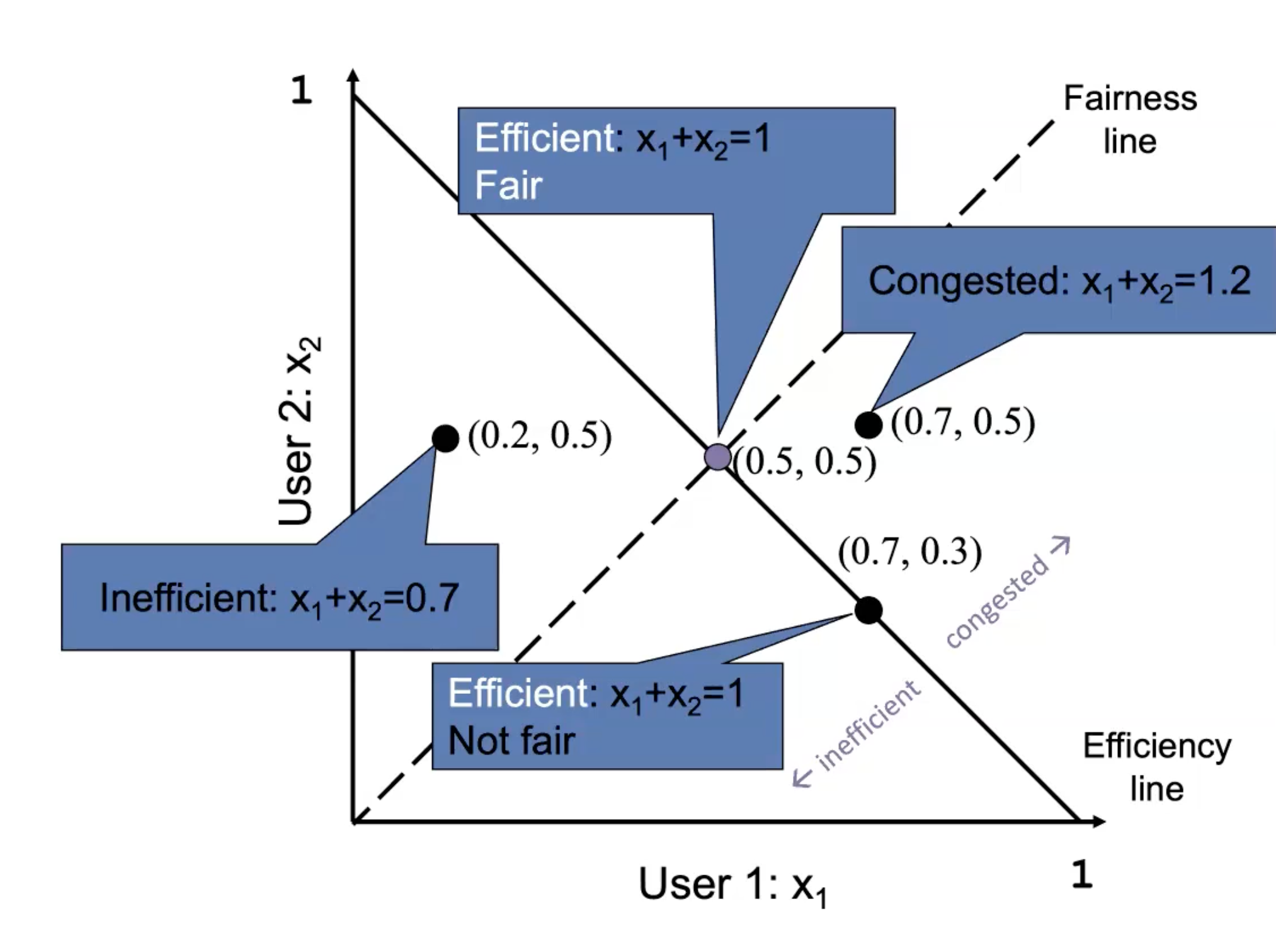
We adjust such that we address the three issues. Recall the last issue is that we are sharing bandwidth, so as we do this we need to balance efficiency (high utilization of link bandwidth; as much capacity as possible) with fairness (each flow gets equal share; don't exhaust others). How do we adjust?

• at every RTT, we can do one of the following
  • multiplicative increase or decrease: CWND $\rightarrow$ a*CWND.
  • additive increase or decrease: CWND $\rightarrow$ CWND + b
• The four alternatives are:
  • AIAD: gentle increase, gentle decrease. This method does not converge to the fairness because it can only move in a diagonal (like parallel to y=x). $x_k+a_i$ or $x_k-a_d$ where $x_k$ is each user, and $a_d$ and $a_i$ are static constants for all users.
  • AIMD: gentle increase, drastic decrease. This is ideal because we get closer to the target point. This is the one used in TCP.
  • MIAD: drastic increase, gentle decrease. This method does not converge to fairness nor efficiency. Imagine multiplication moves along the line created from point to origin, and addition moves along y=x, then it kind of goes away from the fairness line.
  • MIMD: drastic increase, drastic decrease. This method does not converge to fairness because we are moving along one dimension similar to AIAD.

What is fair and efficient?

AIMD

• additive increase
  • for each ACK, CWND = CWND + 1/CWND
  • CWND is increased by one only if all segments in CWND have been acknowledged.
• multiplicative decrease:
  • on packet loss, divide ssthersh in half and slow start. So, ssthresh = CWND/2 and CWND = 1.
  • we're ignoring the dupAck fix for now

Implementation

Congestion control implementation:

• States at the sender
  • CWND is first initialized to a small constant
  • ssthresh is initailized to a large constant
  • dupACKcount and timer
• The events and their reaction as sub-bullets
  • ACK of new data. When this happen, there are two options:
    • If CWND < ssthresh, this means we are in slow start. Increase CWND += 1 (note: this is doubling RTT). This is called the slow start phase.
    • Else we are in the congestion avoidance phase: CWND = CWND + 1/CWND (note: there is a CWND packet per RTT, so by doing this, after one RTT with no drops, CWND = CWND + 1).
  • dupACK which is duplicate ACK for old data
    • We have a counter, that we increment: dupACKcount++
    • if dupACKcount == 3, this is fast retransmit (what dupACKcount == 1 mean is potentially just a reordering, so we want to really make sure there's been a loss). This means we should set sshtresh = CWND/2, and we update CWND = CWND/2
  • Timeout means there is a complete loss. This is serious, so we decrease the rate drastically:
    • ssthresh $\leftarrow$ CWND/2 and CWND $\leftarrow$ 1. By setting the ssthresh to this value, we are taking advantage of knowing the previous value of CWND, and then restart slow-start knowing this.

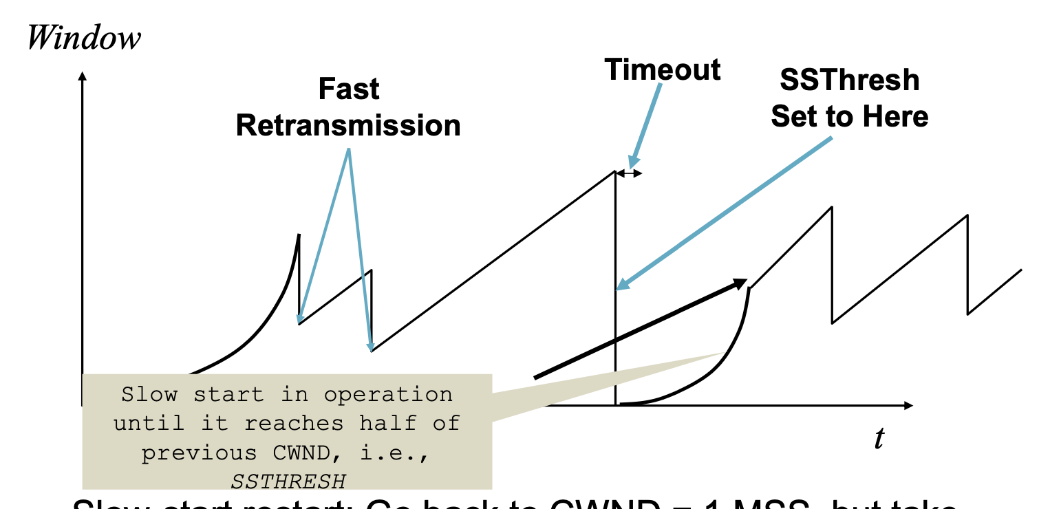
Fast Recovery

There's still a problem: congestion avoidance is too slow in recovering from an isolated loss. For example, consider CWND = 10, and the last ACK was packet #101 i.e., receiver is expecting next packet to have seq no 101. 10 packets are in flight ([101, 102, ..., 110]) but packet 101 is dropped. The timeline of what the receiver sends is:

• ACK 101 (due to 102) cwnd = 10 dupACK#1 (no xmit)
• ACK 101 (due to 103) cwnd = 10 dupACK#2 (no xmit)
• ACK 101 (due to 104) cwnd = 10 dupACK#3 (no xmit)
• retransmit 101 ssthresh = 5, cwnd = 5
• ACK 101 (due to 105) cwnd = 5 (no xmit)
• ACK 101 (due to 106) cwnd = 5 (no xmit)
• ACK 101 (due to 107) cwnd = 5 (no xmit)
• ACK 101 (due to 108) cwnd = 5 (no xmit)
• ACK 101 (due to 109) cwnd = 5 (no xmit)
• ACK 101 (due to 110) cwnd = 5 (no xmit)
• ACK 111 (due to 101) $\leftarrow$ only now we can transmit new packets.
• plus no packets in flight so ACK "clocking" to increase CWND stalls for another RTT.

The solution to this is fast recovery: grant the sender temporary "credit" for each dupACK so as to keep packets in flight. If dupACKcount = 3, then ssthresh = CWND/2, and CWND = ssthresh+3

• This means that while in fast recovery, the CWND = CWND + 1 for each additional dupACK
• Exit fast recovery after receiving the new ACK by setting CWND = ssthresh.

Let's look at the same example as above:

• ACK 101 (due to 102) cwnd = 10 dupACK#1 (no xmit)
• ACK 101 (due to 103) cwnd = 10 dupACK#2 (no xmit)
• ACK 101 (due to 104) cwnd = 10 dupACK#3 (no xmit)
• retransmit 101 ssthresh = 5, cwnd = 5 + 3 = 8
• ACK 101 (due to 105) cwnd = 9 (no xmit) (anytime we get a dup ACK, we keep adding 1 to CW)
• ACK 101 (due to 106) cwnd = 10 (no xmit) (still no transmit because we already have 10 packets in flight. Only transmit when we have less packets in flight than the CW)
• ACK 101 (due to 107) cwnd = 11 (xmit 111)
• ACK 101 (due to 108) cwnd = 12 (xmit 112)
• ACK 101 (due to 109) cwnd = 13 (xmit 113)
• ACK 101 (due to 110) cwnd = 14 (xmit 114)
• ACK 111 (due to 101) cwnd = 5 (xmit 115) ($\leftarrow$ this is where we exit fast recovery and we set CWND = ssthresh)
• Now, packets 111-114 are already in flights.
• ACK 112 (due to 111) cwnd = 5 + 1/5 ($\leftarrow$ we are back in congestion avoidance)

Other TCP Flavors

TCP Flavors:

• TCP-Tahoe: CWND = 1 on 3 dupACKs,
• TCP-Reno: CWND = 1 on timeout, CWND = CWND/2 on 3 dupACKs
• TCP-newReno: TCP-Reno + improved fast recovery (our default option)
• TCP-SACK: incorporates selective acknowledgements

How can different TCP flavors coexist?

• this is because they all follow the same principle: which is to increase CWND on good news and decrease on bad news.