Routers

IP Routers are the core building block of the internet infrastructure. It's a $120B+ industry. Vendors include Cisco, Huawei, Juniper, Nokia (accounts for >90%).

Router Capacity is $N \times R$, where $N$ is the number of external router "ports" and $R$ is the speed, or "line rate" of a port.

Types of router:

• Core has R = 10/40/100 Gbps, NR = O(100) Tbps (aggregated)
• Edge (ISP) has R = 1/10/40 Gbps, NR = O(100) Gbps
• Homes, small business have R = 10/100/1000Mbps, NR < 10 Gbps

Internals

Diagram of what's in a router:

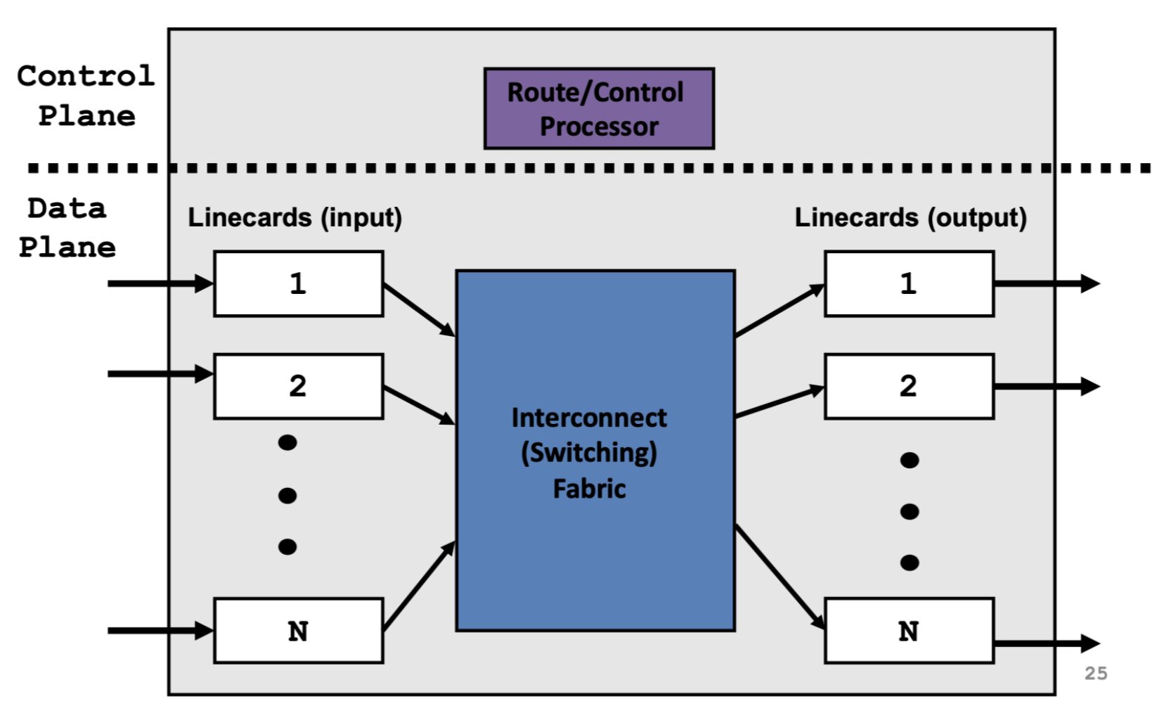
Linecards: Input linecards process packets on the way in and output linecards process packets on the way out. The input and output for the same port are on the same physical linecard.

Interconnect/switching fabric transfers packets from input to output ports, and there's variety of ways to do this.

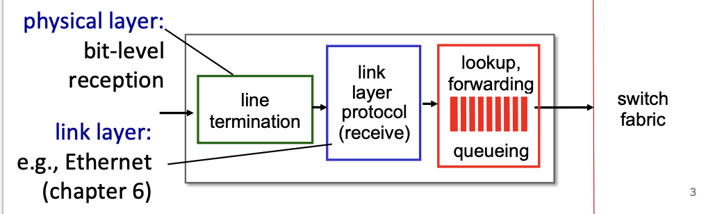
Input Linecards and LPM

Input linecards are in charge of the following tasks:

• receive input packets (physical layer stuff)
• update packer header like TTL, checksum, options, and fragment (easy)
• lookup on destination address (harder)
• queue the packet at the switch fabric
• The main challenge is processing speeds. E.g., 100B packets at 40Gbps means that a new packet arrives every 20ns. It's implemented with specialized hardware (ASICs network processors) so that it can be super fast.
  • Hardware implementations are not disclosed because that's what the companies sell
  • Software implementations are slower but allow immediate updates

How do we find the output port? What if one address maps to multiple ports?

• one entry for each address means that there would be 4 billion entries. For scalability, addresses are aggregated (aggregate means you can divide by the number of ports). This means that a router with 4 ports would map a destination address range to each one.
• E.g.,
  • Port 1 responsible for 11 00 00 00 to 11 00 00 11.
  • Port 2 responsible for 11 00 01 00 to 11 00 01 11.
  • Port 3 responsible for 11 00 10 00 to 11 00 11 11.
  • Port 4 responsible for 11 01 00 00 to 11 01 11 11.

One method is to test each entry to find a match. This scales poorly, and takes O(n)

Leverage a tree structure of binary strings.

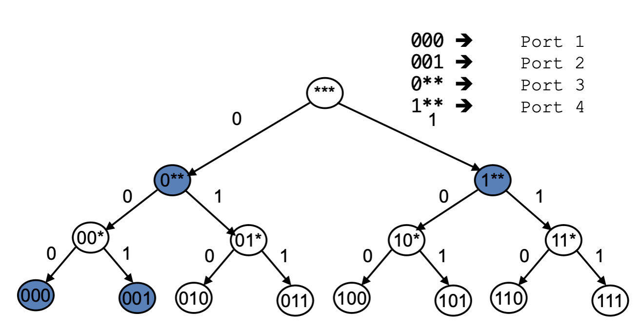• Record the port associated with the latest match, and only override when it matches another prefix during walk down tree.

Longest Prefix Match (LPM). Each packets has a destination IP address, so the router looks up table entry that matches the longest prefix match.

• I.e., matches with the one with most pre-defined values

Switching Fabric

Switching fabric: transfer packet from input link to the appropriate output link. There should be N input ports and N output ports. There are three primary ways to switch:

• switching via shared memory
• switching via a bus
• switching via a inter-connection network. For example, cross bar

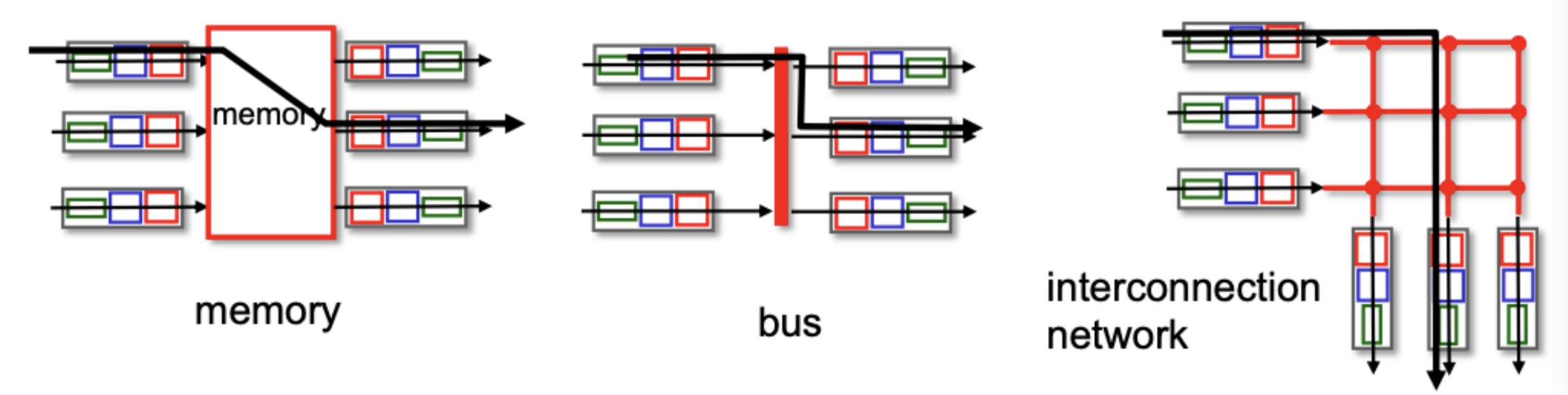
Switching rate is the rate at which packets can be transferred from inputs to outputs. Ideally its NR.

Switching via shared memory means that the packet copied to system's memory, then the memory (this is where the mapping is done) is sent to the desired output.

• this was done in first generation routers. Traditional computers with switching under direct control of CPU.
• speed is limited by memory bandwidth (2 bus crossing per datagram).

Switching via bus: datagram moves from input port memory (input port does the mapping) to output port memory via a shared bus.

• bus contention: switching speed limited by bus bandwidth.
• 32 Gbps bus, Cisco 5600: sufficient speed for access routers.

Switching via interconnection network:

• crossbar
• central scheduler
• initially developed to connect processors in multiprocessor
• scheduling formulated as finding a matching on a bipartite graph.
• practical solutions look for a good maximal matching (fast).

Input port queuing: if switch fabric is slower than input ports combined, then queuing may occur at input queues.

• queueing delay and loss is due to input buffer overflow.

Head-of-the-Line (HOL) blocking: queued datagram at front of the queue prevents others in the queue from moving forwards.

Output Linecards

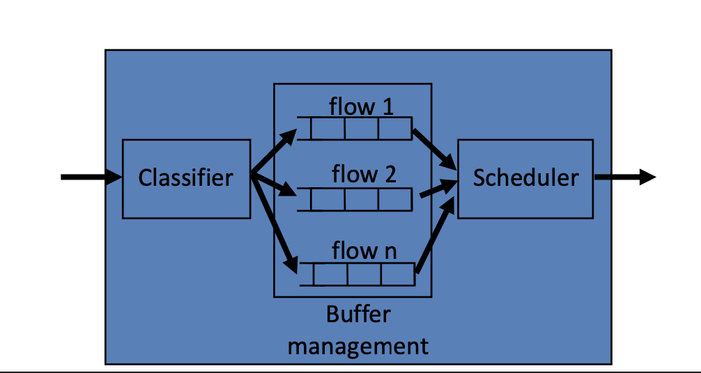
Output linecards:

• packet classification: map packets to flows
• buffer management: decide when and which packet to drop
• scheduler: decide when and which packet to transmit
• (some of these functionalities can also be implemented at input linecards)

Buffer management

Buffer management is in charge of two aspects.

• drop: which packet to drop when buffers are full. There are two techniques:
  • tail drop: drop the arriving packets
  • head drop: drop the packet at the head
  • priority: drop/remove on priority basis
• marking: which packets to mark (ECN, RED). This shows that there is a congestion building up

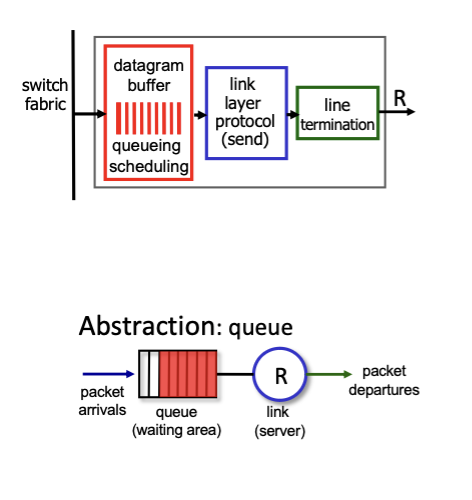
Network is best effort, there's no guarantee, that's why they drop packets.

Packet scheduling: deciding which packet to send on next link. There are a variety of scheduling priorities:

• first come, first served
• priority
• round robin
• weighted fair queueing

FCFS: packets transmitted in order of arrival to output port. Also known as first-in-first-out (FIFO).

Packet classification: classify an IP packet based on a number of fields in the packet header. The scheduler can use this data to determine priority between classes. Examples of different classes:

• source/destination IP address (32 bit)
• source/destination TCP port number (16 bits)
• type of service (TOS) byte (8 bits)
• type of protocol (8 bits)

Packet Scheduling Policies

Let's explore the packet scheduling policies:

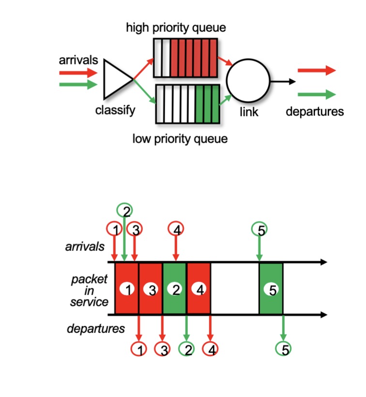
Priority: arriving traffic classified, queue them base on class. Send the packet from the highest priority queue that has buffered packets (within priority class, choose first come first serve).

• Any header field can be used for classification.
• Problem: it could starve the one with the lower priority because we will always deprioritze.

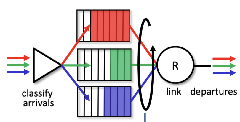
Round robin (RR) scheduling policy: arriving traffic is classified, queued by class. Server cyclically and repeatedly scans class queues, sending one complete packet from each class (if available) in turn.

• Any header field can used for classification
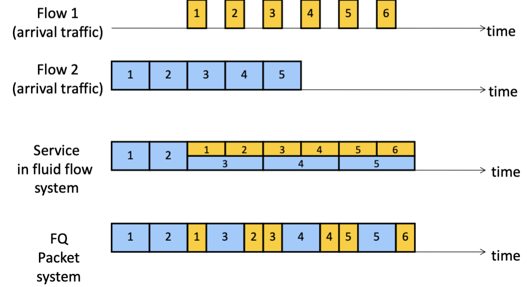
• One concern comes from how packets are of different sizes. Small packets will take little time but big packets will take a long time, resulting in inequality. Bit-by-bot round robin ("fluid flow") is hard to do in practice because packets cannot be preempted. However, we can approximate it with "fair queuing".

Fair queuing (FQ) uses one queue per packet flow and services them in rotation, such that each flow can obtain an equal fraction of the resources. Implementation of round-robin generalized to the case where not all packets are equal sized. Example:

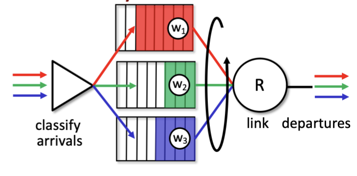
Weighted fair queuing (WFQ): assigns different flows different shares. Each class, $i$, has weight $w_i$, and gets weighted amount of service in each cycle.

Router-Assisted Congestion Control

Routers are the nodes that actually experience congestion; they know that their queues are building up.

The idea: let congested routers announce the congestion to the sender. There are two general ways:

• out of band notification: where the routers explicitly sends pause frames upstream. Requires you to form a packet and send it, which may cause more congestion in the network.
• in-band notification: mark the data packet and let the receiver inform the sender via ACK (ECN) and drops packets sooner (RED). Mark the bit in the header of each packet, so that the receiver can indicate to the sender that they need to slow down.

Explicit Congestion Notification

Explicit Congestion Notification (ECN):

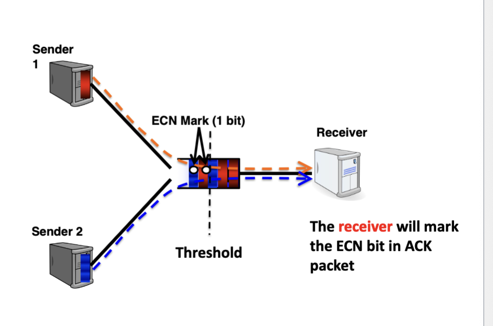
• the ECN mark bit indicates that the network is experiencing congestion. The packet is received by the receiver and when it sees this bit marked, it sends back an ACK with that bit flagged as well in order to communicate this to the sender.

There are many options when routers set the bit.

• there is a tradeoff between (link) utilization and the (packet) delay.

Congestion semantics can be exactly like that of drop

• i.e., end-host reacts as though it saw a drop

ECN Advantages over TCP. Don't confuse corruption with congestion; recovery with rate adjustment. ECN serves as an early indicator of congestion to avoid delay. It's easier to incrementally deploy. Today, its defined in RFC 3168 using ToS/DSCP bits in the IP header. Commonly used in datacenters.

Random Early Detection

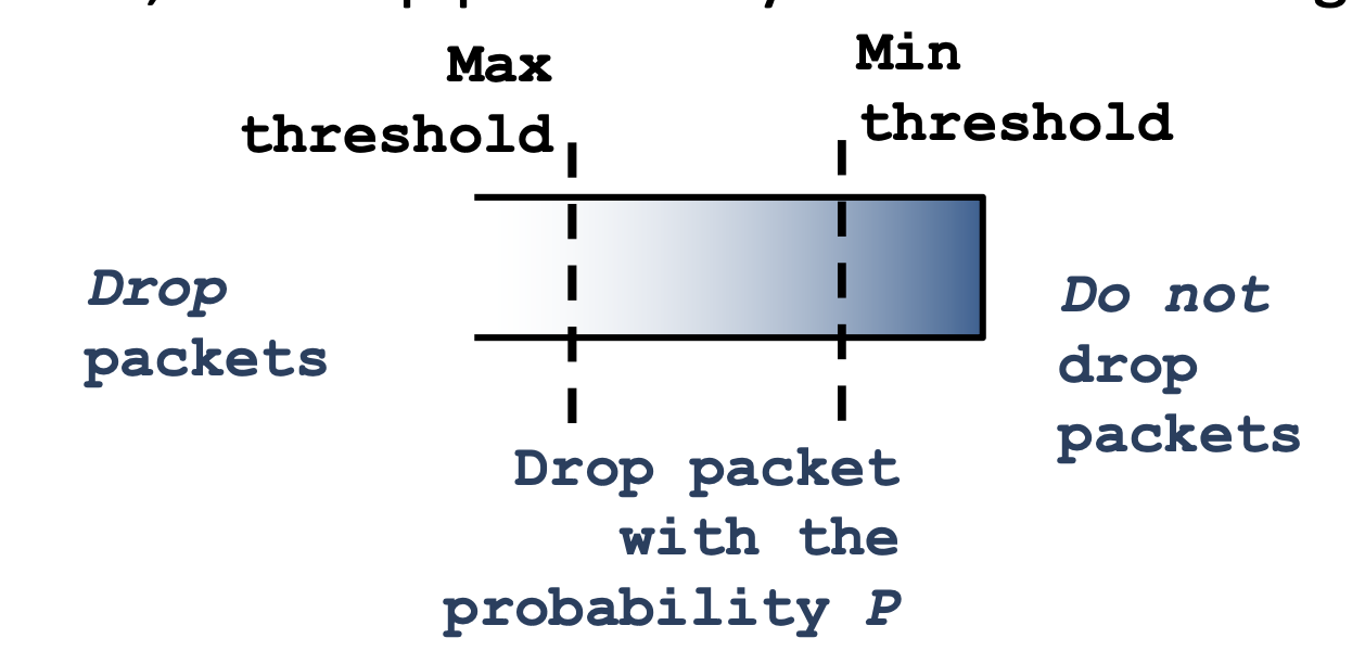
Random Early Detection (RED): the router notices that the queue is getting backlogged, and it randomly drops packets to signal congestion.

• The packet drop probability increases as queue length increases. Otherwise, set drop probability as function of average queue length.
• There's a min threshold, where before this, no packets are dropped. There's also a max threshold, where beyond this, packets are guaranteed to be dropped. However in the middle this is where the packet drop probability $P$ is utilized.

Routing

Recall that

• forwarding is the act of directing a packet to the correct interface so that it progresses to its destination. This is done by reading the address from the packet header and then searching through the forwarding table. Forwarding: "data plane".
• routing is setting up a network-wide forwarding table to enable end-to-end communication by using different routing protocols. Routing: "control plane" is jointly computed by routers using a distributed algorithm.

The goal of routing is finding a path to a given destination. Knowing whether the state contained in the forwarding table meets our goal is called its "validity" (this is not a standard terminology).

Local routing state is the forwarding table in a single router.

• by itself, the state in a single router cannot be evaluated
• must be evaluated in terms of the global context

Global state refers to the collection of forwarding tables in each of the routers.

• It determines which paths packets take.

Validity

A global state is "valid" if it produces a forwarding decisions that always deliver packets to their destination. It is valid if and only if

• There are no dead ends (other than destination). A dead end is when there is no outgoing link (no next-hop). For example, when a packet arrives, the forwarding decision does not yield any outgoing link. E.g., the router doesn't have an "otherwise" row that directs the packet if no matches are found.
• There are no loops. A loop is when a packet cycles around the same set of nods.

How can we tell if routing state is valid? We need a concise correctness condition for routing. The necessary and sufficient condition for a valid global state is listed above. So what is the process of checking validity of routing state?

• focus on a single destination and ignore all the other routing states.
• mark outgoing link ("next hop") with arrow. There is only one at each node
• eliminate all links with no arrow
• look at what's left.

For example,

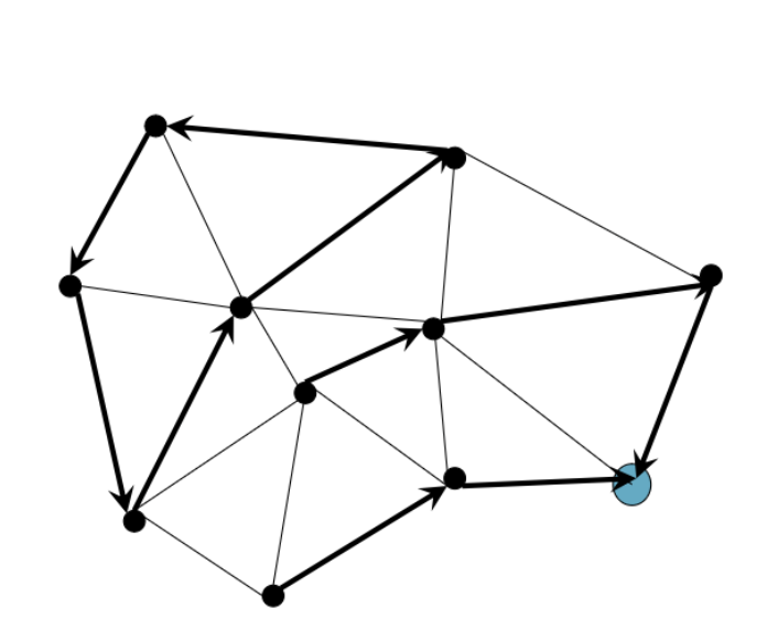
• this is not valid because there is a loop.

Through this method, we can check the validity of a routing state for a particular destination.

• Dead ends are nodes without outgoing arrows
• Loops are obvious and they'll be disconnected from the rest of the graph.

Least-Cost Path Routing

Expanding the goals of routing:

• v1: find a path to a given destination
• v2: find a least-cost path to a given destination

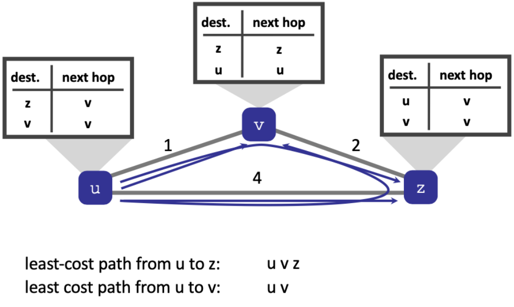
• the direct path from u > z costs 4
• the indirect path from u > v > z costs 3

Least-cost path routing: given a router graph and its link costs, find the least-cost path. This path is from each source router to each destination router.

• provides an easy way to avoid loop because it's not possible for a cost metric is minimized by traversing a loop (it'll have infinite cost).

Dijkstra's Algorithm

Dijkstra's algorithm is a graph search algorithm that finds the shortest path between nodes in a graph with non-negative edge weights.

• the network topology must be known. Network topology is a graph of nodes with the link costs known to all nodes. All nodes should have the same information
• it computes the least-cost paths from one node (the src node) to all the other node.
• takes k iterations to know the least-cost paths to k destinations.
• notation:
  • c(x,y) is the link cost from x to y. Value is $\infty$ if x and y are not direct neighbors
  • D(v) is the current value of cost of path path from source s to dst v
  • p(v) is the predecessor node along path from source s to v (used to create the shortest path)
  • N' is the set of nodes whose least-cost path is definitively known.
• Ties can exist

// Initialization: put cost of u neighbors, otherwise ∞
N' = {u}; D(u) = 0  
For all nodes v  
	if v adjacent to u  
		then D(v) = c(u,v)  
	else D(v) = ∞

// Loop
until all nodes are in N':
	Find w not in N' such that D(w) is a minimum  
	add w to N'  
	update D(v) for all v adjacent to w and not in N':  
	D(v) = min( D(v), D(w) + c(w,v) )  
	/* new cost to v is either old cost to v or known least path cost to w plus cost from w to v */  

Dijkstra's is a local computation as its computed by a node given a complete network graph. Possibilities:

• a separate machine runs the algorithm
• every router runs the algorithm (Internet uses this option)

Link-State Routing

Link-state routing: every router knows its local "link state". E.g., router u: "(u,v) with cost=2; (u,x) with cost=1"

Each router floods its local link state to all other routers in the network periodically or when the link state changes. Every router will learn the entire network graph.

• With this information each router runs Dijkstra's Shortest-path first (SPF) algorithm locally to compute forwarding table.

Flooding is when a node sends its link-state information out to all of its links. The next node forwards this information on all its link except the one the information arrived from. Flooding is initiated in any of the following scenarios:

• topology change (e.g., link/node failure/recovery)
• configuration change (e.g., link cost change)
• periodically to refresh link-state information (soft states), typically every 30 minutes.

We flood because we want all the nodes in the network to converge to the new topology. Upon convergence, all nodes will have consistent routing information and can compute consistent forwarding:

• all nodes have the same link-state database
• all nodes forward packets on shortest paths
• the next router on the path forwards to the expected next hop.

Convergence delay is the time to achieve convergence delay. Other sources include:

• time to detect failure
• time to flood link-state information
• time to re-compute forwarding tables

What would happen if it takes too long to converge? There will be a loop from convergence delay: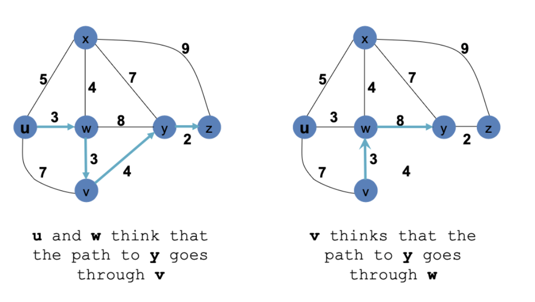

During the convergence period there are a few effects on its performance:

• looping packets
• lost packets due to black holes, which is the situation where network packets are routed to a destination that does not exist or cannot be reached, which results in data loss.
• out-of-order packets reaching the destination.

What is the scalability of link-state routing?

• O(NE) messages
• O(N$^2$) computation time
• O(Network diameter) convergence delay
• O(N) entries in forwarding table

Link-state routing protocols are:

• OSPF: open shortest path first.
  • It's open and publicly available.
  • It uses link-state algorithm. This includes link-state packet dissemination, topology map at each node, route computation using Dijkstra's algorithm.
  • The router floods OSPF link-state advertisement (contain information about the state of links, the cost of reaching different network destinations, and other relevant routing information) to all other routers in entire AS. This is carried in OSPF messages directly in the IP datagram (rather than TCP or UDP). It requires reliable transmission because accuracy of link-state is important.
• IS-IS: intermediate system to intermediate system. It's similar to OSPF.

Distance Vector Routing

While in link-state routing protocol, each node broadcasts its local information, in distance-vector routing protocol, each nodes tell its neighbor about its global view.

• it's kind of the opposite of link-state routing.

The Bellman-Ford equation:

• let $d_x(y) := \text{cost of least-cost path from x to y}$
• then $d_x(y) = \text{min}_v \{c(x,b) + d_v(y)\}$ where we are taking min over all its neighbors $v$ of $x$. $c$ is the cost to neighbor $v$ and $d_v(y)$ is the cost from neighbor $v$ to destination $y$.

Example of bellman-ford: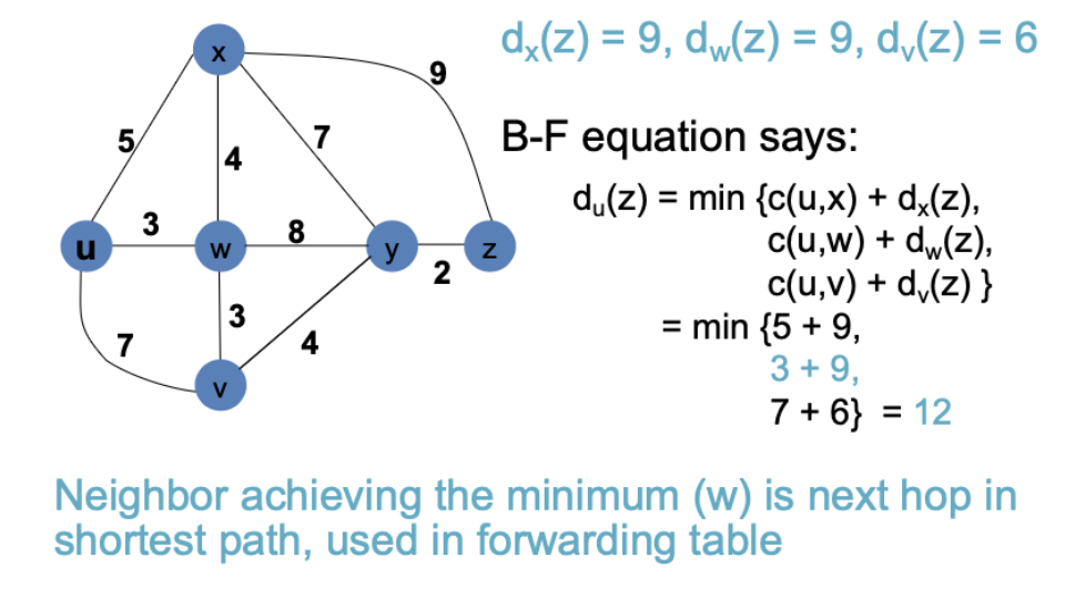

• so now $w$ will be set in the routing table.

Distance vector algorithm: $D_x(y)$ is the estimate of the least cost from $x$ to $y$. $x$ maintains its own distance vector $D_{x} = [D_x(y): t \in N]$

• Node $x$ knows the cost to each neighbor $v$ via $c(x,v)$.
• Node $x$ maintains its neighbor's distance vectors: for each neighbor $v$, $x$ has $D_v=[D_v(y):y \in N]$

From time-to-time, each node sends its own distance vector estimate to its neighbors. When $x$ receives new DV estimate from neighbor, it will update its own DV using the Bellman Ford equation. $D_x(y) \gets min_v \{c(x,b) + D_v(y)\}$ for each node $y \in N$.

• Eventually, the estimate $D_x(y)$ may converge to the actual least cost $d_x(y)$

It's iterative, asynchronous. This means that local iterations is caused by local link cost change or when they receive a DV (distance vector) update message from neighbor.

It's also distributed, meaning that each node notifies neighbors only when its DV change. Neighbors will then notify its neighbors if necessary.

@each node:

1. wait for (change in local link cost or message from its neighbor)
2. recompute estimates
3. notify neighbors if DV to any destination has change.
4. go back to step 1.

Problem with Bellman-ford is that there may be routing loops. For example, z routes through y, and y routes through x. If y loses connectivity to x, then y deicides to route through z. Another problem is that it can take a very long time to resolve, this is called the count-to-infinity scenario.

One heuristic to avoid count-to-infinity is the poisoned reverse:

• if z routes to x through y, then z should advertise to y that its cost to x is infinite.
• y never decides to route to x through z

However, is still not guaranteed. Loop-free routing examples include path vector and source tracing.

Is distance-vector routing scalable?

• requires fewer messages than Link-State
• O(N) update time on arrival of a new DV from neighbor
• O(network diameter) convergence time
• O(N) entries in forwarding table

RIP is a protocol that implements DV (IETF RFC 2080).

Compare link-state and distance-vector routing:

• message complexity:
  • LS with N nodes and E links sends O(NE) messages.
  • DV exchanges between neighbors only
• speed of converges
  • LS is relatively fast
  • DV convergence time varies (count to infinity problem)
• Robustness (what happens if a router malfunctions?)
  • LS node would advertise the incorrect link cost to everyone. Each node computes its own table.
  • DV node can advertise incorrect path cost. Each node's table used by others (error propagates). Since its global, it messes up everyone.
• similarities:
  • both are shortest-path based routing. The common optimization goal is to minimize cost metric (link weights). Routers share a common view as to what makes path "good" and how to measure "goodness"
    • due to a shared goal, its commonly used inside an organization. RIP and OSPF are most used for intra-domain routing.